Transform Data with Julia

import
transform
Tidier.jl
Author
Published

March 10, 2024

Note

This is the second post in the NGSIM data analysis series. Previous post:

After completing this post, you will be able to:
  • Read parquet files
  • Do a quick clean-up of column names
  • Convert integer time to datetime fromat
  • Sort data by columns
  • Create new columns
  • Remove undesired columns
  • Filter data

This post shows code in Julia. You can see the same post written in Python here and in R here.

In the previous post, we partitioned the Interstate 80 (I80) vehicle trajectories data by time and then saved it on disk:

We now make use of the parquet file in the period=first directory for learning to transform data. Since this file is part of partitioned data, I saved it as a separate parquet file (i80_period1.parquet) in a different location.

Load parquet file

Reading the parquet file requires the Parquet2 package:

# ] add Parquet2
using DataFrames
using Parquet2: Dataset
path_to_first_period_file = "data/i80_period1.parquet"
data_jl = DataFrame(Dataset(path_to_first_period_file));

first(data_jl, 5)
5×24 DataFrame
Row Vehicle_ID Frame_ID Total_Frames Global_Time Local_X Local_Y Global_X Global_Y v_length v_Width v_Class v_Vel v_Acc Lane_ID O_Zone D_Zone Int_ID Section_ID Direction Movement Preceding Following Space_Headway Time_Headway
Int32? Int32? Int32? Int64? Float64? Float64? Float64? Float64? Float64? Float64? Int32? Float64? Float64? Int32? Int32? Int32? Int32? Int32? Int32? Int32? Int32? Int32? Float64? Float64?
1 3027 8493 813 1113433984200 53.115 363.266 6.04284e6 2.13343e6 15.3 7.4 2 21.46 -8.14 5 missing missing missing missing missing missing 3014 3032 64.23 2.99
2 3214 9115 708 1113434046400 67.931 655.629 6.04282e6 2.13373e6 13.8 6.3 2 15.37 11.2 6 missing missing missing missing missing missing 3221 3229 31.71 2.06
3 3199 9329 575 1113434067800 17.026 1237.59 6.04268e6 2.1343e6 14.4 5.9 2 39.3 0.0 2 missing missing missing missing missing missing 3188 3206 72.36 1.84
4 3159 8919 572 1113434026800 16.541 306.905 6.04281e6 2.13337e6 16.4 5.9 2 14.71 3.61 2 missing missing missing missing missing missing 3152 3171 51.9 3.53
5 3314 9324 616 1113434067300 28.846 65.807 6.04285e6 2.13314e6 14.8 6.4 2 36.24 0.0 3 missing missing missing missing missing missing 3301 0 103.26 2.85

Clean dataframe names

As you can see above, the column names are in good shape i.e., without any spaces. However, it is easier typing lowercase letters than the sentence case. So, we use the clean_names macro from the TidierData package to make all column names lower case. If the column names have spaces or periods in them, clean_names would replace them with underscores.

using TidierData
data_jl = @clean_names(data_jl)

@glimpse(data_jl)
Rows: 1250932
Columns: 24
.vehicle_id    Union{Missing, Int32}3027, 3214, 3199, 3159, 3314, 3128, 3031, 29
.frame_id      Union{Missing, Int32}8493, 9115, 9329, 8919, 9324, 9052, 9030, 86
.total_frames  Union{Missing, Int32}813, 708, 575, 572, 616, 603, 958, 987, 760,
.global_time   Union{Missing, Int64}1113433984200, 1113434046400, 1113434067800,
.local_x       Union{Missing, Float64}53.115, 67.931, 17.026, 16.541, 28.846, 17
.local_y       Union{Missing, Float64}363.266, 655.629, 1237.592, 306.905, 65.80
.global_x      Union{Missing, Float64}6.042839372e6, 6.042817933e6, 6.042683444e
.global_y      Union{Missing, Float64}2.133434927e6, 2.133726884e6, 2.134296961e
.v_length      Union{Missing, Float64}15.3, 13.8, 14.4, 16.4, 14.8, 16.8, 15.3, 
.v_width       Union{Missing, Float64}7.4, 6.3, 5.9, 5.9, 6.4, 8.5, 7.4, 5.8, 8.
.v_class       Union{Missing, Int32}2, 2, 2, 2, 2, 2, 2, 2, 2, 2, 2, 2, 2, 2, 2,
.v_vel         Union{Missing, Float64}21.46, 15.37, 39.3, 14.71, 36.24, 35.69, 2
.v_acc         Union{Missing, Float64}-8.14, 11.2, 0.0, 3.61, 0.0, 11.2, 10.8, -
.lane_id       Union{Missing, Int32}5, 6, 2, 2, 3, 2, 4, 4, 5, 5, 4, 6, 6, 2, 4,
.o_zone        Union{Missing, Int32}missing, missing, missing, missing, missing,
.d_zone        Union{Missing, Int32}missing, missing, missing, missing, missing,
.int_id        Union{Missing, Int32}missing, missing, missing, missing, missing,
.section_id    Union{Missing, Int32}missing, missing, missing, missing, missing,
.direction     Union{Missing, Int32}missing, missing, missing, missing, missing,
.movement      Union{Missing, Int32}missing, missing, missing, missing, missing,
.preceding     Union{Missing, Int32}3014, 3221, 3188, 3152, 3301, 3125, 0, 2973,
.following     Union{Missing, Int32}3032, 3229, 3206, 3171, 0, 3132, 3032, 2987,
.space_headway Union{Missing, Float64}64.23, 31.71, 72.36, 51.9, 103.26, 90.81, 
.time_headway  Union{Missing, Float64}2.99, 2.06, 1.84, 3.53, 2.85, 2.54, 0.0, 3
The @glimpse macro shows that all variable names are now in lower case now. But variables have the Missing type common. This is perhaps because some of the columns have missing values. Let’s look at 2 variables:

count(x -> ismissing(x), data_jl.frame_id)
0
count(x -> ismissing(x), data_jl.o_zone)
1250932

We therefore remove all the columns that have missing values (completely missing!). Even after that, one of the type of the remaining variables is Missing. So, we replace missing values with zero just to change the type:

data_jl = @select(data_jl, Not(:o_zone, :d_zone, :int_id, :section_id, :direction, :movement))
for col in names(data_jl)
    data_jl[!, col] .= coalesce.(data_jl[!, col], 0)
end

How to create a time column?

Since vehicle trajectories change over time, it is nice to see these changes over different time periods. However, the gloabl_time column in this dataset contains integers rather than the actual time. So, we create a new column called actual_time by dividing the global_time by 1000 and converting it to a datetime object.

In Julia, this can be done via Dates package. The integer to datetime data conversion will report time in UTC. But the data were collected in Los Angeles, so we want to specify the America/Los_Angeles time zone. Thus, we subtract 7 hours as UTC is 7 hours ahead of PDT:

using Dates

data_jl.actual_time = DateTime.(Dates.unix2datetime.(data_jl.global_time ./ 1000))
data_jl.actual_time = data_jl.actual_time .- Hour(7)

first(data_jl, 5)
5×19 DataFrame
Row vehicle_id frame_id total_frames global_time local_x local_y global_x global_y v_length v_width v_class v_vel v_acc lane_id preceding following space_headway time_headway actual_time
Int32 Int32 Int32 Int64 Float64 Float64 Float64 Float64 Float64 Float64 Int32 Float64 Float64 Int32 Int32 Int32 Float64 Float64 DateTime
1 3027 8493 813 1113433984200 53.115 363.266 6.04284e6 2.13343e6 15.3 7.4 2 21.46 -8.14 5 3014 3032 64.23 2.99 2005-04-13T16:13:04.200
2 3214 9115 708 1113434046400 67.931 655.629 6.04282e6 2.13373e6 13.8 6.3 2 15.37 11.2 6 3221 3229 31.71 2.06 2005-04-13T16:14:06.400
3 3199 9329 575 1113434067800 17.026 1237.59 6.04268e6 2.1343e6 14.4 5.9 2 39.3 0.0 2 3188 3206 72.36 1.84 2005-04-13T16:14:27.800
4 3159 8919 572 1113434026800 16.541 306.905 6.04281e6 2.13337e6 16.4 5.9 2 14.71 3.61 2 3152 3171 51.9 3.53 2005-04-13T16:13:46.800
5 3314 9324 616 1113434067300 28.846 65.807 6.04285e6 2.13314e6 14.8 6.4 2 36.24 0.0 3 3301 0 103.26 2.85 2005-04-13T16:14:27.300

Note that the data is not in the correct order. The vehicle_ids in the first two rows are 3027 and 3214. However, we know that the same vehicle was observed for several seconds. This means that we should see a given vehicle_id repeated over multiple rows consecutively. We therefore sort by vehicle_id and frame_id:

## First: Sort by Vehicle ID and Time
data_jl = @arrange(data_jl, vehicle_id, frame_id)
first(data_jl, 5)
5×19 DataFrame
Row vehicle_id frame_id total_frames global_time local_x local_y global_x global_y v_length v_width v_class v_vel v_acc lane_id preceding following space_headway time_headway actual_time
Int32 Int32 Int32 Int64 Float64 Float64 Float64 Float64 Float64 Float64 Int32 Float64 Float64 Int32 Int32 Int32 Float64 Float64 DateTime
1 1 12 884 1113433136100 16.884 48.213 6.04284e6 2.13312e6 14.3 6.4 2 12.5 0.0 2 0 0 0.0 0.0 2005-04-13T15:58:56.100
2 1 13 884 1113433136200 16.938 49.463 6.04284e6 2.13312e6 14.3 6.4 2 12.5 0.0 2 0 0 0.0 0.0 2005-04-13T15:58:56.200
3 1 14 884 1113433136300 16.991 50.712 6.04284e6 2.13312e6 14.3 6.4 2 12.5 0.0 2 0 0 0.0 0.0 2005-04-13T15:58:56.300
4 1 15 884 1113433136400 17.045 51.963 6.04284e6 2.13312e6 14.3 6.4 2 12.5 0.0 2 0 0 0.0 0.0 2005-04-13T15:58:56.400
5 1 16 884 1113433136500 17.098 53.213 6.04284e6 2.13312e6 14.3 6.4 2 12.5 0.0 2 0 0 0.0 0.0 2005-04-13T15:58:56.500

When we want to compare several vehicle trajectories, e.g., how their speeds change over time regardless of when they were observed, we’d want a common time scale. The NGSIM documentation describes that vehicles were observed at a resolution of 0.1 seconds. So, we can create atime variable for each vehicle that starts at 0 and ends at (n-1)/10 where n = number of rows for which a vehicle_id is repeated:

data_jl = @chain data_jl begin
    @group_by(vehicle_id)
    @mutate(time = (0:(first(n()) - 1))/10)
    @ungroup()
end;
1
Group by vehicle_id so that time is calculated for each vehicle separately.
2
n() gives the group size.
3
Don’t forget to ungroup.

How to create variables for the preceding vehicle?

We’d often need velocity, acceleration, and other variables for the preceding vehicle (vehicle in front of the subject vehicle). These variables can be useful in car-following modeling.

In this dataset, preceding vehicle variables do not exist as separate columns. The only relevant column is preceding which is the identifier of the preceding vehicle. But the data also contains the subject vehicle identifier vehicle_id, along with these variables:

  • local_y: longitudinal position of the front end of the subject vehicle (feet)
  • local_x: lateral position of the front end of the subject vehicle (feet)
  • v_length and v_width are the length and width of the subject vehicle (feet)
  • v_class is the class of the subject vehicle, i.e., 1 = motorcycle, 2 = car, and 3 = heavy vehicle (bus/truck)
  • v_vel and v_acc are the velocity (ft/s) and acceleration (ft/s/s) of the subject vehicle

Our goal now is to create new columns of the above variables for the preceding vehicle. To this end, we look for the value of preceding in the vehicle_id column at a given value of frame_id (identifier of time frame) and then grab the value of variable e.g., v_vel at that frame_id. In Julia, we achieve this by joining a few columns of the dataset with the full dataset while using the columns vehicle_id and preceding for the join:

# Join
data_jl = leftjoin(
           data_jl,
           data_jl[:, [:frame_id, :vehicle_id, :local_y, :v_length, :v_width, :v_class, :v_vel, :v_acc]],
           on = [:frame_id => :frame_id, :preceding => :vehicle_id],
           makeunique = true, 
           renamecols = "" => "_preceding"
       )

# Arrange again
data_jl = @arrange(data_jl, vehicle_id, frame_id)


# Rename columns to match with naming in R and Python posts
data_jl = @chain data_jl begin
    @rename(preceding_local_y = local_y_preceding,
            preceding_length =  v_length_preceding,
            preceding_width = v_width_preceding,
            preceding_class = v_class_preceding,
            preceding_vel = v_vel_preceding,
            preceding_acc = v_acc_preceding)
end

first(data_jl, 5)
5×26 DataFrame
Row vehicle_id frame_id total_frames global_time local_x local_y global_x global_y v_length v_width v_class v_vel v_acc lane_id preceding following space_headway time_headway actual_time time preceding_local_y preceding_length preceding_width preceding_class preceding_vel preceding_acc
Int32 Int32 Int32 Int64 Float64 Float64 Float64 Float64 Float64 Float64 Int32 Float64 Float64 Int32 Int32 Int32 Float64 Float64 DateTime Float64 Float64? Float64? Float64? Int32? Float64? Float64?
1 1 12 884 1113433136100 16.884 48.213 6.04284e6 2.13312e6 14.3 6.4 2 12.5 0.0 2 0 0 0.0 0.0 2005-04-13T15:58:56.100 0.0 missing missing missing missing missing missing
2 1 13 884 1113433136200 16.938 49.463 6.04284e6 2.13312e6 14.3 6.4 2 12.5 0.0 2 0 0 0.0 0.0 2005-04-13T15:58:56.200 0.1 missing missing missing missing missing missing
3 1 14 884 1113433136300 16.991 50.712 6.04284e6 2.13312e6 14.3 6.4 2 12.5 0.0 2 0 0 0.0 0.0 2005-04-13T15:58:56.300 0.2 missing missing missing missing missing missing
4 1 15 884 1113433136400 17.045 51.963 6.04284e6 2.13312e6 14.3 6.4 2 12.5 0.0 2 0 0 0.0 0.0 2005-04-13T15:58:56.400 0.3 missing missing missing missing missing missing
5 1 16 884 1113433136500 17.098 53.213 6.04284e6 2.13312e6 14.3 6.4 2 12.5 0.0 2 0 0 0.0 0.0 2005-04-13T15:58:56.500 0.4 missing missing missing missing missing missing

In this dataset, missing indicates that the value is missing because there was no preceding vehicle observed. For vehicle_id 1 we can see this is true because the preceding value is 0.

How to remove undesired columns?

There are several variables in this dataset that we don’t need as they are completely devoid of any value. We have removed those variables already. We further remove variables that we don’t need for analysis:

data_jl = @select(data_jl, Not(:total_frames, starts_with("global"), :following))
first(data_jl, 5)
5×21 DataFrame
Row vehicle_id frame_id local_x local_y v_length v_width v_class v_vel v_acc lane_id preceding space_headway time_headway actual_time time preceding_local_y preceding_length preceding_width preceding_class preceding_vel preceding_acc
Int32 Int32 Float64 Float64 Float64 Float64 Int32 Float64 Float64 Int32 Int32 Float64 Float64 DateTime Float64 Float64? Float64? Float64? Int32? Float64? Float64?
1 1 12 16.884 48.213 14.3 6.4 2 12.5 0.0 2 0 0.0 0.0 2005-04-13T15:58:56.100 0.0 missing missing missing missing missing missing
2 1 13 16.938 49.463 14.3 6.4 2 12.5 0.0 2 0 0.0 0.0 2005-04-13T15:58:56.200 0.1 missing missing missing missing missing missing
3 1 14 16.991 50.712 14.3 6.4 2 12.5 0.0 2 0 0.0 0.0 2005-04-13T15:58:56.300 0.2 missing missing missing missing missing missing
4 1 15 17.045 51.963 14.3 6.4 2 12.5 0.0 2 0 0.0 0.0 2005-04-13T15:58:56.400 0.3 missing missing missing missing missing missing
5 1 16 17.098 53.213 14.3 6.4 2 12.5 0.0 2 0 0.0 0.0 2005-04-13T15:58:56.500 0.4 missing missing missing missing missing missing

How to transform multiple columns?

Metric units

As discussed before, variables in this dataset have imperial units (feet, ft/s, etc.). You may want to transform the values of these variables to metric units. The conversion factor is 0.3048. Here, we write a function to take a column and apply the conversion factor along with rounding to 2 decimal places:

## metric units
function convert_and_round(x)
    return round(x * 0.3048, digits=2)
end

cols_to_mutate = ["local_x", "local_y", "v_length", "v_width", 
                 "v_vel", "v_acc", "space_headway",
                 "preceding_local_y", "preceding_length", "preceding_width",
                 "preceding_vel", "preceding_acc"]

for col in cols_to_mutate
    data_jl[!, col] .= convert_and_round.(data_jl[!, col])
end

first(data_jl, 5)
5×21 DataFrame
Row vehicle_id frame_id local_x local_y v_length v_width v_class v_vel v_acc lane_id preceding space_headway time_headway actual_time time preceding_local_y preceding_length preceding_width preceding_class preceding_vel preceding_acc
Int32 Int32 Float64 Float64 Float64 Float64 Int32 Float64 Float64 Int32 Int32 Float64 Float64 DateTime Float64 Float64? Float64? Float64? Int32? Float64? Float64?
1 1 12 5.15 14.7 4.36 1.95 2 3.81 0.0 2 0 0.0 0.0 2005-04-13T15:58:56.100 0.0 missing missing missing missing missing missing
2 1 13 5.16 15.08 4.36 1.95 2 3.81 0.0 2 0 0.0 0.0 2005-04-13T15:58:56.200 0.1 missing missing missing missing missing missing
3 1 14 5.18 15.46 4.36 1.95 2 3.81 0.0 2 0 0.0 0.0 2005-04-13T15:58:56.300 0.2 missing missing missing missing missing missing
4 1 15 5.2 15.84 4.36 1.95 2 3.81 0.0 2 0 0.0 0.0 2005-04-13T15:58:56.400 0.3 missing missing missing missing missing missing
5 1 16 5.21 16.22 4.36 1.95 2 3.81 0.0 2 0 0.0 0.0 2005-04-13T15:58:56.500 0.4 missing missing missing missing missing missing

Convert numbers to string data type

Moreover, we know that there are variables that should be treated as categorical (qualitative) rather than numbers. For instance, lane_id has values 1-7 and we know that these are identifiers for lanes. Similarly, the class of a vehicle is encoded as 1, 2, and 3 but we know that these numbers do not have any quantitaive information, rather they are categories.

We use the string function to convert numbers to string data type:

data_jl[!,:vehicle_id] = string.(data_jl[!,:vehicle_id])
data_jl[!,:v_class] = string.(data_jl[!,:v_class])
data_jl[!,:lane_id] = string.(data_jl[!,:lane_id])
data_jl[!,:preceding] = string.(data_jl[!,:preceding])
data_jl[!,:preceding_class] = string.(data_jl[!,:preceding_class])

first(data_jl, 5)
5×21 DataFrame
Row vehicle_id frame_id local_x local_y v_length v_width v_class v_vel v_acc lane_id preceding space_headway time_headway actual_time time preceding_local_y preceding_length preceding_width preceding_class preceding_vel preceding_acc
String Int32 Float64 Float64 Float64 Float64 String Float64 Float64 String String Float64 Float64 DateTime Float64 Float64? Float64? Float64? String Float64? Float64?
1 1 12 5.15 14.7 4.36 1.95 2 3.81 0.0 2 0 0.0 0.0 2005-04-13T15:58:56.100 0.0 missing missing missing missing missing missing
2 1 13 5.16 15.08 4.36 1.95 2 3.81 0.0 2 0 0.0 0.0 2005-04-13T15:58:56.200 0.1 missing missing missing missing missing missing
3 1 14 5.18 15.46 4.36 1.95 2 3.81 0.0 2 0 0.0 0.0 2005-04-13T15:58:56.300 0.2 missing missing missing missing missing missing
4 1 15 5.2 15.84 4.36 1.95 2 3.81 0.0 2 0 0.0 0.0 2005-04-13T15:58:56.400 0.3 missing missing missing missing missing missing
5 1 16 5.21 16.22 4.36 1.95 2 3.81 0.0 2 0 0.0 0.0 2005-04-13T15:58:56.500 0.4 missing missing missing missing missing missing

Visualization with one vehicle

Cool! We are almost done with transforming our dataset. It is time to do some visualization. The last transformation we learn is to filter the data to keep only one vehicle:

data_jl_veh = @filter(data_jl, vehicle_id == "2");

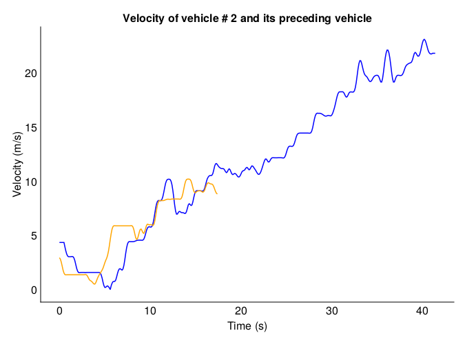
And now we use TidierPlots to create a plot of velocity over time. Subject vehicle in blue and preceding vehicle in orange.

using TidierPlots
ggplot(data = data_jl_veh) +
  geom_path(aes(x = "time", y = "v_vel"), color = "blue") +
  geom_path(aes(x = "time", y = "preceding_vel"), color = "orange") +
  labs(x = "Time (s)", y = "Velocity (m/s)",
       title = "Velocity of vehicle # 2 and its preceding vehicle") +
  theme_minimal()
height: 400
x: Time (s)
title: Velocity of vehicle # 2 and its preceding vehicle
width: 600
y: Velocity (m/s)

geom_path
data: inherits from plot
x: time 
y: v_vel 

geom_path
data: inherits from plot
x: time 
y: preceding_vel 

ggplot options
data: A DataFrame (415 rows, 21 columns)

As you see, the lead vehicle speed is not seen after about 17 seconds. This is because the lead vehicle changed lanes.

Reuse

Citation

BibTeX citation:
@online{durrani2024,
  author = {Durrani, Umair},
  title = {Transform {Data} with {Julia}},
  date = {2024-03-10},
  langid = {en}
}
For attribution, please cite this work as:
Durrani, Umair. 2024. “Transform Data with Julia.” March 10, 2024.